from matplotlib import pyplot as plt
import numpy as np

TaperMixin - Controlling onset and offset of functions

This mixin is included in every non-AnalyticFunctionGenerator classes in letalker to apply smooth on/off patterns both easily and flexibly.

In this demo, we employ ConstantGenerator class to illustrate the various effect of the TaperMixin.

import numpy as np
from letalker.function_generators import Constant
from letalker.constants import fs

The TaperMixin introduces 4 keyword arguments to the constructor of the supported classes:

• transition_time: float | Sequence[float] | None = None

• transition_type: StepTypeLiteral | Sequence[StepTypeLiteral] = "raised_cos"

• transition_time_constant: float | Sequence[float] = 0.002

• transition_initial_on: bool = False

Let’s examine the effect of each keyword.

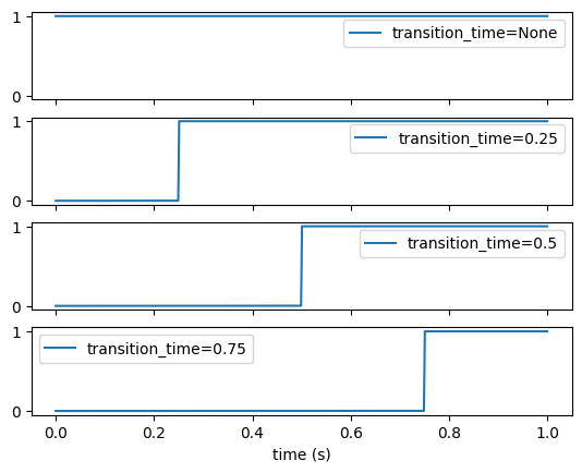
transition_time - Time in seconds at when the transition occurs

By default the taper effect is turned off (i.e., transition_time = None). By assigning a time value to this argument turns on the waveform at this time.

n = fs  # 1 second demo
t = np.arange(n) / fs

cgen0 = Constant(1)
cgen1 = Constant(1, transition_time=0.25)
cgen2 = Constant(1, transition_time=0.5)
cgen3 = Constant(1, transition_time=0.75)

fig, axes = plt.subplots(4, 1, sharex=True, sharey=True)
axes[0].plot(t, cgen0(n, force_time_axis='tile_data'), label="transition_time=None")
axes[0].legend()
axes[1].plot(t, cgen1(n), label="transition_time=0.25")
axes[1].legend()
axes[2].plot(t, cgen2(n), label="transition_time=0.5")
axes[2].legend()
axes[3].plot(t, cgen3(n), label="transition_time=0.75")
axes[3].legend()
axes[3].set_xlabel("time (s)")

Text(0.5, 0, 'time (s)')

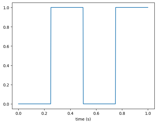
A list of time points could also be assigned to transition_time keyword to generate an on/off sequence.

cgen = Constant(1, transition_time=[0.25, 0.5, 0.75])

plt.plot(t, cgen(n))
plt.xlabel("time (s)")

Text(0.5, 0, 'time (s)')

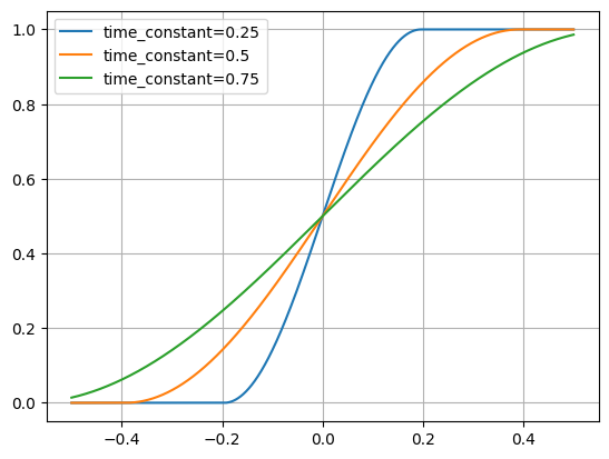
transition_time_constant - Sets the transition duration

This parameter indicates the duration for a linear transition. Other transitions (excluding step) are slower (see below). Default is 0.002 s, matching LeTalker’s respiratory pressure (PL) transition.

for tc in [0.25, 0.5, 0.75]:
    cgen = Constant(1, transition_time=0, transition_time_constant=tc)
    plt.plot(t - 0.5, cgen(n, -n // 2), label=f"time_constant={tc}")
plt.legend()
plt.grid()

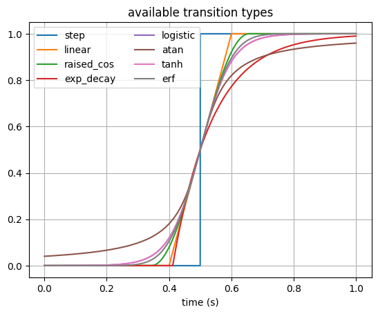
transition_type - Sets the transition waveform

Default is the raised cosine ("raised_cos"), and you may pick one of 6 possibilities:

value	description
"step"	instantaneous transition
"linear"	linear transition
"raised_cos"	raised cosine transition
"exp_decay"	transition of a first-order linear system
"logistic"	logistic function transition
"atan"	arctangent transition
"tanh"	hyperbolic tangent transition
"erf"	error function transition

t = np.arange(0, n) / fs

for ttype in [
    "step",
    "linear",
    "raised_cos",
    "exp_decay",
    "logistic",
    "atan",
    "tanh",
    "erf",
]:
    cgen = Constant(
        1, transition_type=ttype, transition_time=0.5, transition_time_constant=0.2
    )
    plt.plot(t, cgen(n), label=ttype)
plt.legend(ncols=2)
plt.title("available transition types")
plt.xlabel("time (s)")
plt.grid()

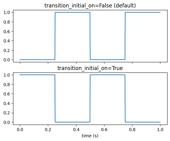
transition_initial_on

Setting transition_initial_on = True makes the first transition to turn off the signal.

cgen0 = Constant(1, transition_time=[0.25, 0.5, 0.75], transition_initial_on=False)
cgen1 = Constant(1, transition_time=[0.25, 0.5, 0.75], transition_initial_on=True)

fig, axes = plt.subplots(2, 1, sharex=True, sharey=True)
axes[0].plot(cgen0.ts(n), cgen0(n), label="initial_on=False (default)")
axes[0].set_title("transition_initial_on=False (default)")
axes[1].plot(cgen0.ts(n), cgen1(n), label="initial_on=True")
axes[1].set_title("transition_initial_on=True")
axes[1].set_xlabel("time (s)")

Text(0.5, 0, 'time (s)')